

If you have ever stared at a machine learning paper and hit a wall the moment you see P(x|y), you are not alone. Probability is the language most ML algorithms are written in, and skipping it means guessing why your model works instead of knowing. This guide breaks down the seven probability concepts for machine learning you actually need, with plain explanations and real examples instead of textbook jargon.
Random Variables and Probability Distributions
A random variable is just a rule that assigns a number to the outcome of something uncertain. Flip a coin and call heads 1, tails 0. That is a random variable. A probability distribution then tells you how likely each outcome is.
In machine learning, this shows up everywhere. When a classifier outputs [0.83, 0.12, 0.05] for three classes, it is describing a probability distribution over possible labels. When you generate text with an LLM, the model is sampling from a probability distribution over the next token.
Two types matter most:
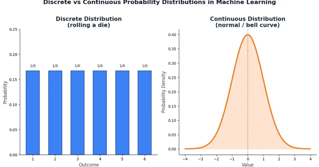
- Discrete distributions (Bernoulli, Binomial, Categorical) handle countable outcomes like classes or coin flips
- Continuous distributions (Normal, Uniform, Exponential) handle measurements like height, pixel intensity, or time between events
Common mistake: treating a softmax output as “the model’s confidence” without understanding it is a probability distribution shaped by training data, not a measure of truth. A model can be very confident and very wrong. Calibration techniques exist specifically because raw softmax probabilities are often overconfident.
Practical tip: whenever you see a model output that sums to 1, ask what distribution it is modeling and what assumptions that distribution makes. That single habit saves hours of debugging weird model behavior later.
Bayes’ Theorem and Conditional Probability
Conditional probability answers one question: given that something already happened, how likely is something else? Bayes’ theorem flips that question around, and it is the backbone of a huge chunk of machine learning.
The formula looks intimidating but the idea is simple:
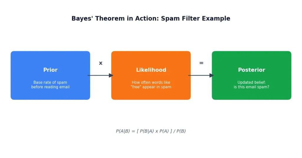
P(A|B) = [P(B|A) x P(A)] / P(B)
Translate that into plain English: your updated belief about A, after seeing evidence B, depends on how likely that evidence is if A were true, multiplied by how likely A was to begin with.
This is exactly how a spam filter works. Before reading an email, there’s a base rate of spam (the prior). After spotting words like “free” and “winner,” the filter updates that belief (the posterior) using how often those words appear in spam versus legitimate mail (the likelihood).
Naive Bayes classifiers, Bayesian optimization for hyperparameter tuning, and even the reasoning behind A/B test significance all lean on this same logic.
Direct takeaway: if you only learn one formula from this entire article, learn Bayes’ theorem. It shows up in spam detection, medical diagnosis models, recommendation systems, and Bayesian neural networks. Skipping it means you are memorizing algorithms instead of understanding why they work.
“All models are wrong, but some are useful.” This applies directly to priors in Bayesian thinking. A prior does not need to be perfect. It needs to be a reasonable starting point that gets corrected by evidence.
The Normal (Gaussian) Distribution
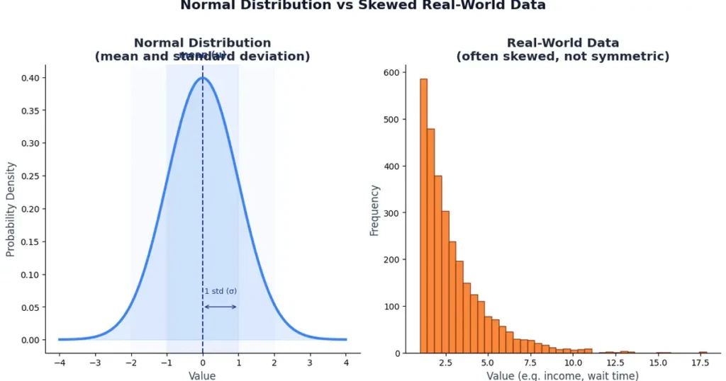
The normal distribution is the bell curve you have seen a hundred times, and it earns its fame because of the Central Limit Theorem: when you average enough independent random variables, the result tends toward a normal distribution, regardless of the original distribution shape.
In ML, this shows up in:
- Weight initialization in neural networks, where weights are often sampled from a normal distribution to keep gradients stable early in training
- Gaussian Naive Bayes, which assumes continuous features follow a normal distribution within each class
- Noise modeling in generative models like diffusion models, which literally learn to reverse a process of adding Gaussian noise
- Linear regression assumptions, where residuals are assumed to be normally distributed for confidence intervals to be valid
A normal distribution is fully described by just two numbers: its mean (center) and standard deviation (spread). That efficiency is exactly why so many algorithms default to assuming normality, even when real data is messier.
Common mistake: assuming your data is normally distributed just because it looks roughly bell-shaped. Real-world data (income, website traffic, word frequency) is often skewed or heavy-tailed. Always check with a histogram or a Q-Q plot before an algorithm that assumes normality.
Expectation, Variance, and Covariance
Expectation (the mean) tells you the average outcome you would expect over many repetitions. Variance tells you how spread out those outcomes are. Covariance tells you how two variables move together.
These three ideas quietly power loss functions. Mean Squared Error is, at its core, the expected squared difference between predictions and actual values. When you compute the variance of your model’s predictions across different training runs, you are directly measuring one half of the bias-variance tradeoff, the concept that explains why an overly complex model overfits and an overly simple one underfits.
Covariance matters even more once you touch:
- Principal Component Analysis (PCA), which relies entirely on the covariance matrix of your features to find directions of maximum variance
- Portfolio-style feature selection, where you want features that are predictive but not redundant with each other
Practical tip: before running PCA or any dimensionality reduction, always look at the covariance (or correlation) matrix first. If two features have near-perfect covariance, one of them is often just noise dressed up as a separate feature.
Maximum Likelihood Estimation (MLE)
Maximum Likelihood Estimation is the method behind training most machine learning models, even if the name never comes up in your code. The idea: given your observed data, find the model parameters that make that data most probable.
Logistic regression, linear regression (under a Gaussian noise assumption), and the cross-entropy loss used to train nearly every neural network classifier are all instances of MLE in disguise. When you minimize cross-entropy loss, you are maximizing the likelihood of the correct labels under your model’s predicted distribution. Same math, different name.
This matters because it explains why loss functions are shaped the way they are. Cross-entropy is not an arbitrary penalty. It is the negative log-likelihood, and negative log-likelihood is what falls out of MLE when your outputs are probabilities.
Direct takeaway: the next time you choose a loss function, ask what probability distribution it implicitly assumes about your data. Mean Squared Error assumes Gaussian noise. Cross-entropy assumes a categorical distribution. Picking the wrong loss for your data’s actual noise pattern quietly hurts performance in ways that are hard to diagnose.
Entropy and KL Divergence
Entropy measures uncertainty. A fair coin flip has high entropy because you cannot predict the outcome. A coin that always lands heads has zero entropy because there is no uncertainty at all.
In machine learning, entropy shows up in:
- Decision trees, where splits are chosen to reduce entropy (or its close cousin, Gini impurity) at each node
- Cross-entropy loss, which measures the gap between your model’s predicted distribution and the true label distribution
KL divergence (Kullback-Leibler divergence) takes this further by measuring how one probability distribution differs from another. It is not symmetric, meaning the “distance” from distribution A to B is not the same as from B to A, and that asymmetry is intentional. It reflects how surprised you would be using distribution B to describe events that actually come from distribution A.
This shows up directly in:
- Variational Autoencoders (VAEs), where KL divergence keeps the learned latent space close to a chosen prior distribution
- Knowledge distillation, where a smaller “student” model learns by minimizing KL divergence between its outputs and a larger “teacher” model’s outputs
- Reinforcement learning from human feedback (RLHF), where KL divergence prevents a fine-tuned model from drifting too far from its original behavior
Common mistake: treating KL divergence as a normal distance metric. Because it is asymmetric, swapping the order of the two distributions in your formula gives a different, often very different, result. Get the order backwards and your model optimizes for the wrong thing entirely.
Joint, Marginal, and Independence
Joint probability is the likelihood of two or more things happening together, written P(A, B). Marginal probability strips one variable away to look at a single event on its own, P(A), by summing or integrating over all possibilities of the other variable. Independence is the special case where knowing one variable tells you nothing about the other, meaning P(A, B) = P(A) x P(B).
This trio matters most in:
- Naive Bayes classifiers, which assume features are conditionally independent given the class, a simplification that is almost never technically true but works surprisingly well in practice
- Graphical models and Bayesian networks, which are essentially a visual map of which variables are dependent on which
- Feature engineering, where checking for independence helps you avoid feeding a model two features that are really just saying the same thing twice
Practical tip: when someone tells you Naive Bayes “assumes independence,” do not treat that as a weakness to apologize for. It is a deliberate trade-off. You give up some accuracy in exchange for a model that trains fast, needs little data, and is easy to interpret. For many real-world text classification tasks, that trade is worth it.
FAQ
Do I need advanced math to understand probability for machine learning?
No. You need a solid grip on the seven concepts above and how to apply them, not a full statistics degree. Most practitioners learn this through applied examples rather than pure theory.
What is the difference between probability and statistics in ML?
Probability is the framework for reasoning about uncertainty before you see data. Statistics is what you use to draw conclusions from data you already have. Machine learning constantly moves between the two.
Is Bayes’ theorem actually used in modern deep learning?
Yes, though often indirectly. Bayesian neural networks, uncertainty estimation, and techniques like dropout as Bayesian approximation all rely on it, and the intuition behind priors and updates shows up in how practitioners reason about model confidence.
Why does cross-entropy loss involve logarithms?
Because cross-entropy comes from negative log-likelihood in Maximum Likelihood Estimation. The logarithm converts a product of probabilities into a sum, which is far easier to optimize and avoids numerical underflow from multiplying many small numbers.
What is the single most useful probability concept for beginners?
Bayes’ theorem, without question. It reframes how you think about evidence and belief, and that mental model pays off across almost every ML algorithm you will encounter next.
Do I need to memorize probability distribution formulas?
No. Understanding which distribution fits which type of data, and why, matters far more than memorizing the formulas. You can always look up the formula. You cannot look up the intuition in the middle of debugging a model.
Conclusion
Probability is not a prerequisite you check off once and forget. It is the reasoning system underneath loss functions, model outputs, and the training process itself. The seven probability concepts for machine learning covered here, random variables and distributions, Bayes’ theorem, the normal distribution, expectation and variance, MLE, entropy and KL divergence, and joint probability, show up again and again once you start looking for them.
Your next step: pick one concept from this list that you understood the least, and find one real model or algorithm where it plays a direct role. Understanding sticks far better when it is tied to something you can actually see working.
- [Source: Stanford CS229 Machine Learning Course Notes on Probability | https://cs229.stanford.edu/]
- [Source: Deep Learning Book by Goodfellow, Bengio, and Courville, Chapter 3: Probability and Information Theory | https://www.deeplearningbook.org/]

Sandeep Kumar is the Founder & CEO of Aitude, a leading AI tools, research, and tutorial platform dedicated to empowering learners, researchers, and innovators. Under his leadership, Aitude has become a go-to resource for those seeking the latest in artificial intelligence, machine learning, computer vision, and development strategies.