Non-linear Independent Components Estimation is a normalizing flow-based generative model which is used to learn the probability distribution of the real samples and then generate the new sample data. This algorithm can be categorized as generative models as GAN and VAE but using a different approach conceptually. While GAN doesn’t impose a prior distribution and VAE approximates the prior distribution, This NICE algorithm estimates the real distribution to which real data belongs. This tutorial is a step-by-step guide to understand the non-linear independent components estimation algorithm and write the code using Tensorflow 2.0.
Introduction
In the normalizing flow method, The probability distribution p(x) is a composition of differentiable bijective functions f.
p(x) = f_0 * f_1*f_2*f_3 .... f_kHere each function f should have following characteristics –
- Easy to differentiable
- Easy to compute the determinant of Jacobian of function f
- And f should be invertible.
The objective of the NICE model is to learn these factorial functions f using a neural network and then use these model training parameters to generate new data. The loss criteria are maximum log-likelihood using the change of variable equation.
log P_X(x) = log P_z(f(x)) + log(\vert det( \frac{\partial(f(x))}{\partial(x)} ) \vert)Here P_z( f(x)) is a prior distribution and \frac{\partial(f(x))}{\partial(x)} is Jacobian matrix of function f at x.
So we’re trying to represent the complex non-linear distribution as a simpler prior distribution.
The NICE model has Coupling Layer and Scaling Layer as the main components in its architecture.
Coupling Layer
The NICE model has multiple coupling layer and each coupling layer represent a function f. So f_0 ,f_1, f_2, f_3 .... f_k are coupling layers. if X is input to a coupling layer then output Y is defined where:
y1 = x1 y2 = g(x2; m(x1))Here x1 and x2 are partitions of the input X and function m is a non-linear neural network.
The Jacobian of f at x is defined as below:
\begin{bmatrix} \frac{\partial y1}{\partial x1}&\frac{\partial y1}{\partial x2} \\ \frac{\partial y2}{\partial x1}&\frac{\partial y2}{\partial x2} \end{bmatrix}In this tutorial, we use additive coupling layer as g function.
y1 = x1 y2 = x2 + m(x1)Note that y2 depends on both x1 and x2 but y1 only depends on x1. so The Jacobian will be:
\begin{bmatrix}1&0 \\ \frac{\partial y2}{\partial x1}&1 \end{bmatrix}This is a lower triangle matrix hence its determinate will be the product of the diagonal elements. so Jacobian of additive coupling layer will be 1 always hence it’s a volume-preserving operation.
Each coupling layer unchanged some part of the input so we combine multiple coupling layers so all inputs elements can be modified.
Scaling Layer
The additive coupling layer is a volume-preserving operation so the composition of all coupling layers will also be a volume-preserving operation which is a problem in a real-life data transformation. Without changing volume of a unknown complex distribution, we can’t transform it to a much simpler distribution. So we introduce a new layer as the output layer of the NICE model architecture which allows us to give more weights to some dimensions and less to others hence more weight variations. So we add a diagonal layer S which transforms the output of coupling layers.
(x_i)_{i<=D} \to (S_{ii}x_i)_{i<=D}NICE Model Architecture
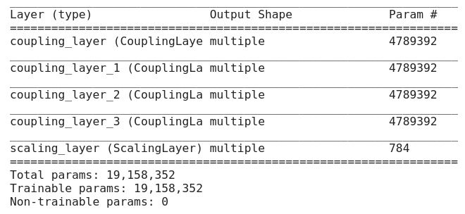
This is the last part we need to discuss before start writing the code. In this tutorial, we’ll use MNIST database as training input and will have following architectural decisions.
- It has 4 Coupling Layers. Each coupling layer consists of Sequential Model which has 1000 units in hidden layers.
- It has 1 scaling layer consists of [1,784] random values from a uniform distribution.
- Maximum loglikelihood as loss function.
- Adam optimizer to update the parameters in backpropagation.
TensorFlow 2.0 Code
Below is the step-by-step guide to implementing the Non-Linear Independent Components Estimation algorithm with TensorFlow. Each line is well commented.
First thing first, load the require libraries.
import tensorflow as tf
from tensorflow import keras
from tensorflow.keras import layers
from tensorflow.keras.datasets import mnist
import numpy as np
import matplotlib.pyplot as plt
Define Coupling Layer
class CouplingLayer(layers.Layer):

	""" This method define the neural network to learn function F

    Parameters
    ----------
    input_dim : int
        - Number of Pixels - width * height
    hidden_dim : int
        - Number of Units per hidden layer
    partition : String
        - Odd or even indexing scheme
    num_layers : int
        - Number of hidden layer

    """

	def __init__(self,input_dim, hidden_dim, partition, num_hidden_layers):

		super(CouplingLayer, self).__init__()

		assert input_dim % 2 == 0

		self.partition = partition # Posssible values - odd or even

		# Define Neural Network

		inputs = keras.Input(shape = (input_dim))

		x = inputs
		for layer in range(num_hidden_layers):
			x = layers.Dense(hidden_dim)(x)
			x = layers.LeakyReLU()(x)

		outputs = layers.Dense(input_dim, activation='linear')(x)
		self.m = keras.Model( inputs = inputs, outputs = outputs)

		# Define lambda functions to get odd or even indexed data.
		if self.partition == 'even':
			self._first = lambda xs: xs[:,0::2]
			self._second = lambda xs: xs[:,1::2]
		else:
			self._first = lambda xs: xs[:,1::2]
			self._second = lambda xs: xs[:,0::2]

	""" This method implement additive coupling layer operations.
	y1 = x1
	y2 = x2 + m(x1)

    Parameters
    ----------
    inputs : Tensor Array
        Input Tensors.

    Returns
        -------
        Tensor Array
            Latent representation.
    """

	def call(self,inputs):

		# Split input into two parts x1 and x2
		x1 = self._first(inputs)
		x2 = self._second(inputs)

		# Inference latent representation
		y1 = x1
		y2 = x2 + self.m(x1)

		# Merge both y1 an y2 using interleave method. e.g y1 = [1,3,5,7,9] and y2 = [2,4,6,8,10] then y = [1,2,3,4,5,6,7,8,9,10]
		if self.partition == 'even':
		      y = tf.reshape(tf.concat([y1[...,tf.newaxis], y2[...,tf.newaxis]], axis=-1), [tf.shape(y1)[0],-1])
		else:
		      y = tf.reshape(tf.concat([y2[...,tf.newaxis], y1[...,tf.newaxis]], axis=-1), [tf.shape(y2)[0],-1])
		return y

	"""This function will generate new image using latent variable

    Parameters
    ----------
    latent_variable : Tensor Array
       . latent variable from logistic distribution.

    Returns
    -------
    List
        Pixels value.
    """
	def inverse(self,latent_variable):

		y1 = self._first(latent_variable)
		y2 = self._second(latent_variable)
		x1,x2 = y1, y2 - self.m(y1)

		if self.partition == 'even':
		      x = tf.reshape(tf.concat([x1[...,tf.newaxis], x2[...,tf.newaxis]], axis=-1), [tf.shape(x1)[0],-1])
		else:
		      x = tf.reshape(tf.concat([x2[...,tf.newaxis], x1[...,tf.newaxis]], axis=-1), [tf.shape(x2)[0],-1])

		return x
Define Scaling Layer
class ScalingLayer(layers.Layer):
	""" This method define the scaling layer with normal distribution.

	Parameters
	----------
	input_dim : int
	- Number of Pixels - width * height
	"""
	def __init__(self,input_dim):
		super(ScalingLayer,self).__init__()
		self.scaling_layer = tf.Variable(tf.random.normal([input_dim]),trainable=True)

	""" This method rescale the final out of coupling layers.

	Parameters
	----------
	x : Tensor Array
	- Tensors to be rescale.
	"""
	def call(self,x):
		return x*tf.transpose(tf.math.exp(self.scaling_layer))

	""" This method is inverse implementation of the call method.

	Parameters
	----------
	z : Tensor Array
	    - Tensors to be rescale.
	"""
	def inverse(self,z):
	    return z*tf.transpose(tf.math.exp(-self.scaling_layer))
Define NICE Model
class NICE(keras.Model):

	""" This function define trainable model with multiple coupling layers and a scaling layer.

    Parameters
    ----------
    input_dim : int
        - Number of Pixels - width * height
    hidden_dim : int
        - Number of Units per hidden layer
    num_hidden_layers : int
        - Number of hidden layer

    """

	def __init__(self,input_dim,hidden_dim,num_hidden_layers):

		super(NICE,self).__init__()
		self.input_dim = input_dim
		# Coupling layer will have half dimension of the input data.
		half_dim = int(self.input_dim / 2)

		# Define 4 coupling layers.
		self.coupling_layer1 = CouplingLayer(input_dim=half_dim, hidden_dim = hidden_dim, partition='odd', num_hidden_layers=num_hidden_layers)
		self.coupling_layer2 = CouplingLayer(input_dim=half_dim, hidden_dim = hidden_dim, partition='even', num_hidden_layers=num_hidden_layers)
		self.coupling_layer3 = CouplingLayer(input_dim=half_dim, hidden_dim = hidden_dim, partition='odd', num_hidden_layers=num_hidden_layers)
		self.coupling_layer4 = CouplingLayer(input_dim=half_dim, hidden_dim = hidden_dim, partition='even', num_hidden_layers=num_hidden_layers)

		# Define scaling layer which rescaling the output for more weight variations.
		self.scaling_layer = ScalingLayer(self.input_dim)

	"""This function calculates the log likelihood.

    Parameters
    ----------
    z : Tensor Array
        Latent space representation.

    Returns
        -------
        List
            Log likelihood.
    """

	def log_likelihood(self, z):
		log_likelihood = tf.reduce_sum(-(tf.math.softplus(z) + tf.math.softplus(-z)), axis=1) + tf.reduce_sum(self.scaling_layer.scaling_layer)
		return log_likelihood

	""" This function passes input through coupling layer. Scale the output using scaling layer and return latent space z and loglikelihood

    Parameters
    ----------
    x : Tensor Array
        Input data from training samples.

    Returns
        -------
        Tensor Array
            Latent space representation.
        List
        	Log-likelihood for each image in the batch
    """

	def call(self, x):

		z = self.coupling_layer1(x)
		z = self.coupling_layer2(z)
		z = self.coupling_layer3(z)
		z = self.coupling_layer4(z)
		z = self.scaling_layer(z)

		log_likelihood = self.log_likelihood(z)
		return z,log_likelihood

	""" Generate sample data using latent space. This is exact inverse of the call method.

    Parameters
    ----------
    z : Tensor Array
        Latent Spaec.

    Returns
    -------
    Tensor Array
        Newly generated data
    """

	def inverse(self,z):
		x  = z
		x  = self.scaling_layer.inverse(x)
		x  = self.coupling_layer4.inverse(x)
		x  = self.coupling_layer3.inverse(x)
		x  = self.coupling_layer2.inverse(x)
		x  = self.coupling_layer1.inverse(x)

		return x

	""" Sample out new data from learnt probability distribution

    Parameters
    ----------
    num_samples : int
        - Number of sample images to generate.

    Returns
    -------
    List
    	- List of generated sample data.

    """

	def sample(self, num_samples):
		z = tf.random.uniform([num_samples, self.input_dim])
		z = tf.math.log(z) - tf.math.log(1.-z)
		return self.inverse(z)
Train NICE Model
Basic model configurations.
input_data_size = 784 # for mnist dataset. 28*28
num_epochs = 100
batch_size = 256
num_hidden_layer = 5
num_hidden_units = 1000
Prepare training dataset.
# Prepare training dataset
(x_train, y_train), (x_test, y_test) = mnist.load_data()
x_train = (x_train.reshape(-1,input_data_size) + tf.random.uniform([input_data_size])) / 256.0
dataloader = tf.data.Dataset.from_tensor_slices((x_train, y_train)).batch(batch_size)
Define a function show_samples() to generate sample images after certain epochs.
def show_samples():
    # Generate 100 sample digits
    ys = model.sample(21)
    plt.figure(figsize=(5, 5))
    plt.rcParams.update({
        "grid.color": "black",
        "figure.facecolor": "black",
        "figure.edgecolor": "black",
        "savefig.facecolor": "black",
        "savefig.edgecolor": "black"})
    new_images = tf.reshape(ys,(-1,28,28))
    for i in range(1,20):
      plt.subplot(2,10,i)
      plt.axis('off')
      plt.imshow(new_images[i],cmap="gray")
    plt.show()
Start custom training loop now.
model = NICE(input_dim = input_data_size, hidden_dim = num_hidden_units, num_hidden_layers = num_hidden_layer)
opt = keras.optimizers.Adam(learning_rate=0.001,clipnorm=1.0)
# Iterate through training epoch
for i in range(num_epochs):
# Iterate through dataloader
for batch_id,(x,_) in enumerate(dataloader):
# Forward Pass
with tf.GradientTape() as tape:
z, likelihood = model(x)
log_likelihood_loss = tf.reduce_mean(likelihood)
# Convert the maximum likelihood problem into negative of minimum likelihood problem
loss = -log_likelihood_loss
# Backward Pass
gradient = tape.gradient(loss,model.trainable_weights)
opt.apply_gradients(zip(gradient,model.trainable_weights))
# Log the maxmimum likelihood after each training loop
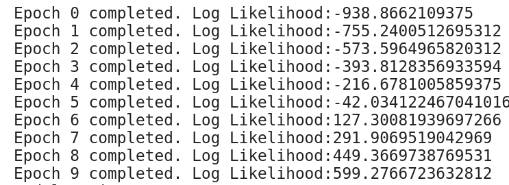
print('Epoch {} completed. Log Likelihood:{}'.format(i,log_likelihood_loss))
# Generate 20 new images after 10 epochs.
if i % 10 == 0 and i!=0:
show_samples()Here are the log of first 10 epochs.
Please read the original paper for a depth understanding. and here is the Github repo Non-Linear Independent Components Estimation with Tensorflow to start playing with the code.

Sandeep Kumar is the Founder & CEO of Aitude, a leading AI tools, research, and tutorial platform dedicated to empowering learners, researchers, and innovators. Under his leadership, Aitude has become a go-to resource for those seeking the latest in artificial intelligence, machine learning, computer vision, and development strategies.