How to Program Generative Adversarial Network with Tensorflow 2.0

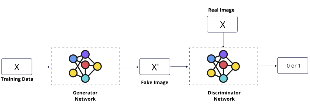
This guide is a hands-on tutorial to program a generative adversarial network with TensorFlow 2.0 to generate new data using the past data. We need to train two networks, Generator, and Discriminator, using alternative approach where for each batch, we train the discriminator first such that it identifies if a provided sample data is fake or real and the generator is trained to generate a new sample data such that discriminator can be fooled to identify a generated sample data as a real data.

Below is the illustration of how a generative adversarial network work.

Step 1 – Prepare Training Data

Load the required libraries.

import tensorflow as tf
from tensorflow import keras
from tensorflow.keras import layers
import numpy as np
import matplotlib.pyplot as plt

Create a two dimensional training array of the size (1024,2)

train_data_length = 1024
x = 2 * np.pi * np.random.rand(train_data_length)
y = np.cos(x)
train_data = np.stack((x,y), axis=1)

Visualize the real dataset we’re using for this tutorial.

plt.title("Real Data Distribution")
plt.plot(train_data[:,0],train_data[:,1],".")
plt.show();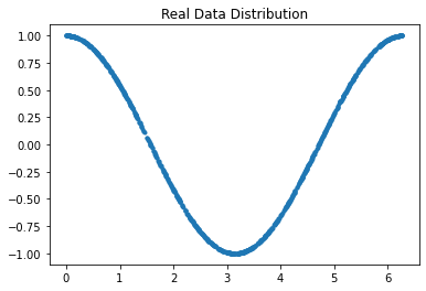

Step 2 – Discriminator Neural Network

For the discriminator neural network, This is a binary classification problem that outputs 0 for Fake Image and 1 for the Real Image so we’ll use the BinaryCrossEntropy activation function at the output layer. For the Input, A two dimensional array will be passed to the Input layer.

discriminator = keras.Sequential([

			keras.Input(shape=(2), name="Input_Layer"),
			layers.Dense(256, activation='relu',name="First_Dense_Layer"),
			layers.Dropout(.3, name="Dropout_1"),
			layers.Dense(128, activation='relu',name="Second_Dense_Layer"),
			layers.Dropout(.3,name="Dropout_2"),
			layers.Dense(64, activation = 'relu',name="Third_Dense_Layer"),
			layers.Dropout(.3,name="Dropout_3"),
			layers.Dense(1, activation='sigmoid',name="Output_Layer")

	],name="Discriminator_Model")

Output the summary of the discriminator model.

discriminator.summary()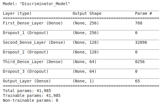

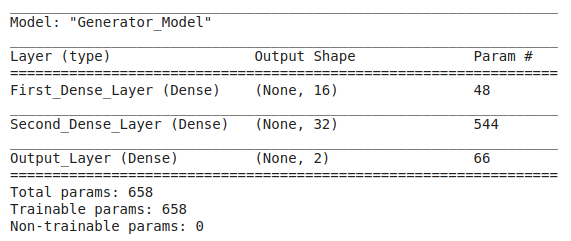
Step 3 – Generator Neural Network

The generator will output the same size of data as input data because our goal is to generate new sample data which distribution is similar to real data distribution. This is a regression problem.

generator = keras.Sequential([

			keras.Input(shape=(2),name="Input_Layer"),
			layers.Dense(16, activation='relu',name="First_Dense_Layer"),
			layers.Dense(32, activation='relu',name="Second_Dense_Layer"),
			layers.Dense(2,name="Output_Layer")

	], name="Generator_Model")

Output the summary of the generator model.

Step 4 – Training Loop

Instead of using the model.fit() or something like this, we’ll create a custom training loop that includes the feed forwarding and backpropagation to train the discriminator and generator.

Below is the complete training loop and each line are commented.

# Configuration
batch_size = 32
epochs = 100
lr = .001

# Prepare Data Pipeline
train_dataset = tf.data.Dataset.from_tensor_slices(train_data).batch(batch_size).shuffle(True)
# Define Loss Function for Discriminator
loss_function = keras.losses.BinaryCrossentropy()
# Define Optimizer for both Discriminator & Generator
dis_optimizer = keras.optimizers.Adam(lr = lr)
gen_optimizer = keras.optimizers.Adam(lr = lr)

# Plot the Generated Data Distribution after 10 epochs. so total we need 10 plots. 

fig, a = plt.subplots(2,5)

j = 0
k = 0
# Start Training Loop
for epoch in range(epochs):
  	# Iterate through training data Data pipeline
	for i, real_samples in enumerate(train_dataset):
		# Define labels for Real Data. All should be 1 because these are real images.
		real_samples_labels = np.ones((batch_size,1))
		# Define a latent space from the normal distribution
		latent_space = np.random.normal(0,1, size = (batch_size,2))
		# Generate Data using Generator Model
		generated_samples = generator(latent_space)
		# Define labels for Generated Data. All should be - because these are fake samples.
		generated_samples_labels = np.zeros((batch_size,1))
		# Contatenate both Real and Generated Data to be passed through discriminator.
		all_samples = np.concatenate((real_samples, generated_samples))
		all_samples_labels = np.concatenate((real_samples_labels, generated_samples_labels))
		
		# Discriminator Training
		with tf.GradientTape() as dis_tape:
			# Forward Propagation
			dis_output = discriminator(all_samples, training = True)
			dis_loss = loss_function(all_samples_labels, dis_output)

		# Backword Propagation
		# Calculate Gradients
		dis_gradients = dis_tape.gradient(dis_loss, discriminator.trainable_weights)
		# Update discriminator parameters
		dis_optimizer.apply_gradients(zip(dis_gradients, discriminator.trainable_weights))

		# Define a latent space from the normal distribution
		latent_space = np.random.normal(0,1, size = (batch_size,2))

		# Generator Training
		with tf.GradientTape() as gen_tape:
			# Forward Propagation
			gen_output  = generator(latent_space, training = True)
				# Pass the fake (generated) data through the discriminator
			dis_output = discriminator(gen_output)
			gen_loss = loss_function(real_samples_labels, dis_output)

		# Backword Propagation
		# Calculate Gradients	
		gen_gradients = gen_tape.gradient(gen_loss, generator.trainable_weights)
		# Update generator parameters
		gen_optimizer.apply_gradients(zip(gen_gradients,generator.trainable_weights))

	# Log losses and Plot the generated data distribution
	if epoch % 10 == 0 and epoch !=0:
		print(f"Discriminator Loss after {epoch} epoch: {dis_loss}")
		print(f"Generator Loss after {epoch} epoch: {gen_loss}")
		latent_space = np.random.normal(0,1, size = (train_data_length,2))
		generated_data = generator(latent_space)

		if j % 5 == 0 and j != 0:
			k = k + 1
			j = 0

		a[k][j].plot(generated_data[:,0], generated_data[:,1],".")
		a[k][j].set_title(f"After {epoch} epoch")
		j = j+1
# Show the grid of generated data distribution
plt.show();

Below are the explanations of this training loop in parts.

Basic Configurations

First define the batch size, learning rate, and the number of epoch. You may do experiments with these parameters.

batch_size = 32
epochs = 100
lr = .001

Data Pipeline

Generate a data pipleline to train the networks over the training data in batches.

train_dataset = tf.data.Dataset.from_tensor_slices(train_data).batch(batch_size).shuffle(True)

Loss & Optimizers

Define the Binary Cross Entropy loss function for the discriminator as this is a binary classification problem.

loss_function = keras.losses.BinaryCrossentropy()

Next, define optimizers for the both network separately.

dis_optimizer = keras.optimizers.Adam(lr = lr)
gen_optimizer = keras.optimizers.Adam(lr = lr)

Discriminator Training

Now start the training loop for certain epochs and iterate through training data in batches for each epoch.

for epoch in range(epochs):
	for i, real_samples in enumerate(train_dataset):

First, create a collection of real and fake samples to be passed as input to the discriminator network.

# Define labels for Real Data. All should be 1 because these are real images.
		real_samples_labels = np.ones((batch_size,1))
		# Define a latent space from the normal distribution
		latent_space = np.random.normal(0,1, size = (batch_size,2))
		# Generate Data using Generator Model
		generated_samples = generator(latent_space)
		# Define labels for Generated Data. All should be - because these are fake samples.
		generated_samples_labels = np.zeros((batch_size,1))
		# Contatenate both Real and Generated Data to be passed through discriminator.
		all_samples = np.concatenate((real_samples, generated_samples))
		all_samples_labels = np.concatenate((real_samples_labels, generated_samples_labels))

Next, feed forward the input through the neural network and calculate the loss.

# Discriminator Training
		with tf.GradientTape() as dis_tape:
			# Forward Propagation
			dis_output = discriminator(all_samples, training = True)
			dis_loss = loss_function(all_samples_labels, dis_output)

Next, for the backpropagation step, calculate the gradients of loss with respect to training parameters and update the parameters using gradient decent.

# Backword Propagation
		# Calculate Gradients
		dis_gradients = dis_tape.gradient(dis_loss, discriminator.trainable_weights)
		# Update discriminator parameters
		dis_optimizer.apply_gradients(zip(dis_gradients, discriminator.trainable_weights))

We have completed Discriminator training part up to now.

Generator Training

For generator neural network training, create a latent space vector to be passed as input for the generator neural network.

latent_space = np.random.normal(0,1, size = (batch_size,2))

For the feed forwarding step, pass the input through the network and calculate the loss. Here is the trick that we pass generated data, the output of the generator, to the Discriminator trained in the previous step and check whether it can identify a generated (fake) sample data as real data or not. Minimum error loss means the discriminator is being a fool.

with tf.GradientTape() as gen_tape:
			# Forward Propagation
			gen_output  = generator(latent_space, training = True)
				# Pass the fake (generated) data through the discriminator
			dis_output = discriminator(gen_output)
			gen_loss = loss_function(real_samples_labels, dis_output)

For backpropagation step, calculate error loss with respect to generator parameters and then update the parameters using gradient decent.

# Calculate Gradients	
		gen_gradients = gen_tape.gradient(gen_loss, generator.trainable_weights)
		# Update generator parameters
		gen_optimizer.apply_gradients(zip(gen_gradients,generator.trainable_weights))

And we have finished the generator training part. now show the loss after 10 epochs and plot the data distribution of generated data.

# Log losses and Plot the generated data distribution
	if epoch % 10 == 0 and epoch !=0:
		print(f"Discriminator Loss after {epoch} epoch: {dis_loss}")
		print(f"Generator Loss after {epoch} epoch: {gen_loss}")
		latent_space = np.random.normal(0,1, size = (train_data_length,2))
		generated_data = generator(latent_space)

		if j % 5 == 0 and j != 0:
			k = k + 1
			j = 0

		a[k][j].plot(generated_data[:,0], generated_data[:,1],".")
		a[k][j].set_title(f"After {epoch} epoch")
		j = j+1

and training loop will be ended here.

At the end show the how data distribution is changing after every 10 epochs.

plt.show()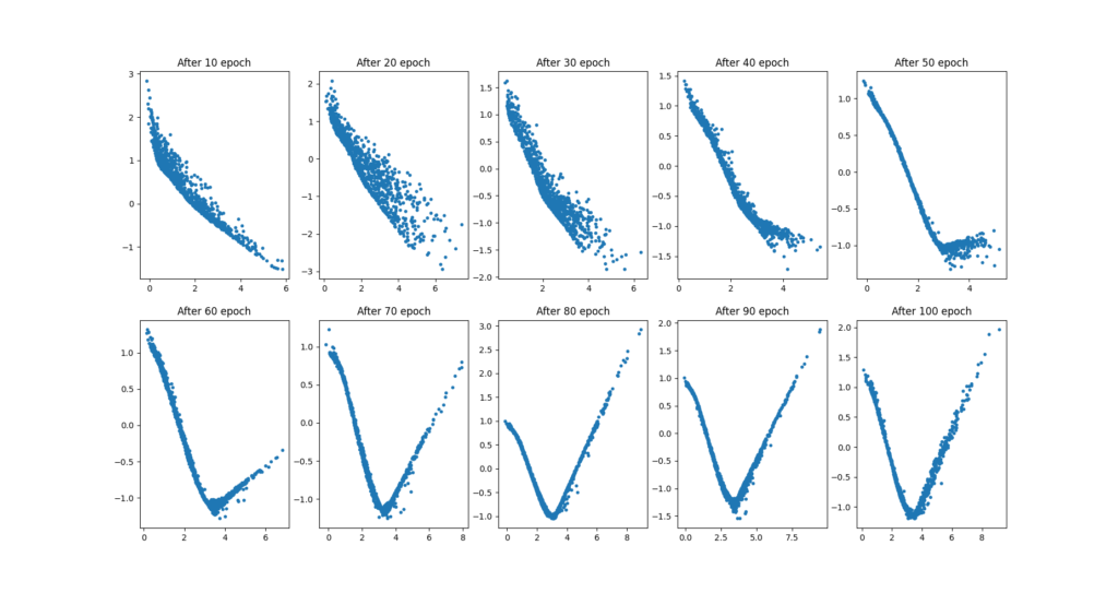

note that at the end of the training, we’re able to generate a data distribution that is similar to our real data distribution.