Decision Tree algorithm belongs to the Supervised Machine Learning. It can use to solve Regression and Classification problems. It creates a training model which predicts the value of target variables by learning decision rules inferred from training data.
- What is Decision Tree?
- Types of Decision Trees
- Important Terminology
- Decision Tree Algorithm Pseudocode
- How do Decision Trees work?
- ID3 Algorithm
- C4.5 Algorithm
- CART Algorithm
- CHAID Algorithm
- MARS Algorithm
- Overfitting
- Advantages of Decision Tree
- Disadvantages of Decision Tree
What is Decision Tree?
It is easy to understand the Decision Trees algorithm compared to other classification algorithms. It solves the problem, by using tree representation. Where each internal node corresponds to an attribute, and each leaf node corresponds to a class label.
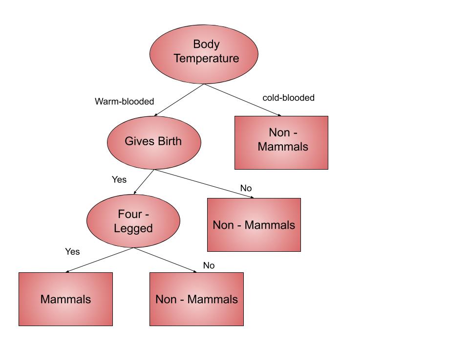
For example, we want to know whether an animal is a mammal or not mammal. given their information like body temperature, gives birth etc. The decision nodes here are questions like ‘Does they give birth’? or ‘how many legs do they have’? And the leaves(outcomes), like either ‘mammals’, or ‘non-mammals’. The above example is a binary classification problem (yes-no type problem).
Types of Decision Trees
We classify Decision Trees into two types:
- Categorical Variable Decision Tree: Here the target variable is of categorical type.
- Continuous Variable Decision Tree: Here the target variable is of continuous type.
Important Terminology
- Root Node: Represents the sample which further gets divided into two or more homogeneous sets.
- Splitting: divides a node into two or more sub-nodes.
- Leaf / Terminal Node: Nodes which do not split is called Leaf or Terminal node.
- Pruning: Removing sub-nodes of a decision node.
- Branch / Sub-Tree: A subset of the entire tree.
- Parent and Child Node: A node which divides into sub-nodes is the parent node. And sub-nodes are the child of a parent node.
Decision Tree Algorithm Pseudocode
- The best attribute of the dataset should be placed at the root of the tree.
- Split the training set into subsets. Each subset should contain data with the same value for an attribute.
- Repeat step 1 & step 2 on each subset. So we find leaf nodes in all the branches of the tree.
For predicting target variable we start from the root of the tree. And then we compare the values of the root attribute with the record’s attribute. After comparison, we follow the branch corresponding to that value and proceed to the next node. We continue comparing until we reach a leaf node with predicted class value.
How do Decision Trees work?
They use multiple algorithms to decide which node to split into two or more sub-nodes. The creation of sub-nodes increases the homogeneity of resultant sub-nodes. The decision tree splits the nodes on all available variables and then choose the split which results in most homogeneous sub-nodes. We select the algorithm on the basis of the type of target variables. Some of the algorithms used in Decision Trees are:
- ID3
- C4.5
- CART(Classification And Regression Tree)
- CHAID(Chi-square automatic interaction detection)
- MARS(multivariate adaptive regression splines)
In this blog, we will read about ID3 Algorithm in detail. As it is the most important and often used algorithm.
ID3 Algorithm
Iterative Dichotomiser 3(ID3) algorithm was invented by J.Ross Quinlan in the year 1975. It generates a decision tree with top-down, greedy search, to test each attribute at every node of the tree. It selects the best attribute that has maximum Information Gain(IG) or minimum Entropy(H). The resultant tree classifies future samples.
For instance, we have been given below a table of a dataset having 14 examples. Here the column Play Tennis is the target variable(label). And other columns such as Outlook, Temperature, Humidity and Wind are the features. We want to know when it is the best Day to play tennis. For this, we want to construct a decision tree for the given training dataset.
| Day | Outlook | Temperature | Humidity | Wind | Play Tennis |
|---|---|---|---|---|---|
| 1 | Sunny | Hot | High | Weak | No |
| 2 | Sunny | Hot | High | Strong | No |
| 3 | Overcast | Hot | High | Weak | Yes |
| 4 | Rain | Mild | High | Weak | Yes |
| 5 | Rain | Cool | Normal | Weak | Yes |
| 6 | Rain | Cool | Normal | Strong | No |
| 7 | Overcast | Cool | Normal | Strong | Yes |
| 8 | Sunny | Mild | High | Weak | No |
| 9 | Sunny | Cool | Normal | Weak | Yes |
| 10 | Rain | Mild | Normal | Weak | Yes |
| 11 | Sunny | Mild | Normal | Strong | Yes |
| 12 | Overcast | Mild | High | Strong | Yes |
| 13 | Overcast | Hot | Normal | Weak | Yes |
| 14 | Rain | Mild | High | Strong | No |
Steps in ID3 Algorithm
- Calculate the entropy for a dataset.
- For each attribute calculate
- Entropy for all its categorical values.
- Information gain for the feature.
- Find the feature having maximum information gain.
- Repeat all the steps until we get the desired decision tree.
Mathematical tools to use
We only need two mathematical tools to implement ID3 Algorithm. This algorithm employs the greedy approach on the dataset. And selects the attribute that yields maximum Information Gain and minimum Entropy.
Entropy
It is the amount of uncertainty in the dataset S. It is mathematically represented as:
Entropy(S) = ∑ – p(I) . log2p(I)
Firstly, we need to calculate Entropy for each and every attribute. The attribute having smallest entropy is used to split the dataset on that particular side. Entropy = 0 signifies all are of the same category.
Information Gain
It means how much uncertainty was reduced in dataset S after splitting S on an attribute A. The attribute having maximum Information Gain is used to split the dataset S on that particular iteration. It is mathematically represented as:
Gain(S, A) = Entropy(S) – ∑ [ p(S|A) . Entropy(S|A) ]
From the dataset, there are 14 entries where 9 out of 14 are “yes” and 5 out of 14 are “no“. Therefore Entropy of the complete dataset is:
H(S) = – p(yes) * log2(p(yes)) – p(no) * log2(p(no))
H(S)= -(9/14) * log2(9/14) – (5/14) * log2(5/14)= 0.94
According to step 2 of pseudocode, we need to calculate Entropy and Information Gain of each attribute.
First Attribute: Outlook
Categorical values= sunny, overcast and rain.
H(Outlook=sunny) = 0.971
H(Outlook=rain) = 0.971
H(Outlook=overcast) = 0
Average Entropy Information for Outlook =
I(Outlook) = p(sunny) * H(Outlook=sunny) + p(rain) * H(Outlook=rain) + p(overcast) * H(Outlook=overcast)
= (5/14)*0.971 + (5/14)*0.971 + (4/14)*0 = 0.693
Information Gain = H(S) – I(Outlook)
= 0.94 – 0.693
= 0.247
Second Attribute – Temperature
Categorical values = hot, mild, cool
H(Temperature=hot) = 1
H(Temperature=cool) = 0.811
H(Temperature=mild) = 0.9179
Average Entropy Information for Temperature =
I(Temperature) = (4/14)*1 + (6/14)*0.9179 + (4/14)*0.811
= 0.9108
Information Gain = H(S) – I(Temperature)
= 0.0292
Third Attribute – Humidity
Categorical values = high, normal
H(Humidity=high) = 0.983
H(Humidity=normal) = 0.591
Average Entropy Information for Humidity =
I(Humidity) = (7/14)*0.983 + (7/14)*0.591
= 0.787
Information Gain = H(S) – I(Humidity)
= 0.94 – 0.787=0.153
Fourth Attribute – Wind
Categorical values = weak, strong
H(Wind=weak) = 0.811
H(Wind=strong) = 1
Average Entropy Information for Wind =
I(Wind)= (8/14)*0.811 + (6/14)*1
= 0.892
Information Gain = H(S) – I(Wind)
= 0.94 – 0.892= 0.048
Now, we know Outlook has the maximum Information Gain. Therefore the decision tree built will be:
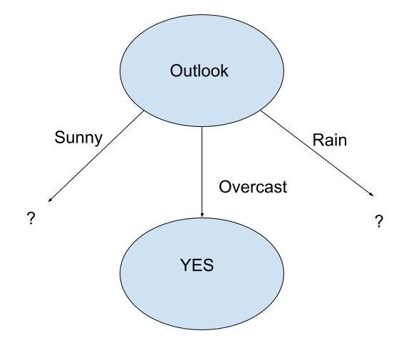
When outlook = Overcast, we have pure class(yes)
| Day | Outlook | Temp. | Humidity | Wind | Play Tennis |
|---|---|---|---|---|---|
| 3 | Overcast | Hot | High | Weak | Yes |
| 7 | Overcast | Cool | Normal | Strong | Yes |
| 12 | Overcast | Mild | High | Strong | Yes |
| 13 | Overcast | Hot | Normal | Weak | Yes |
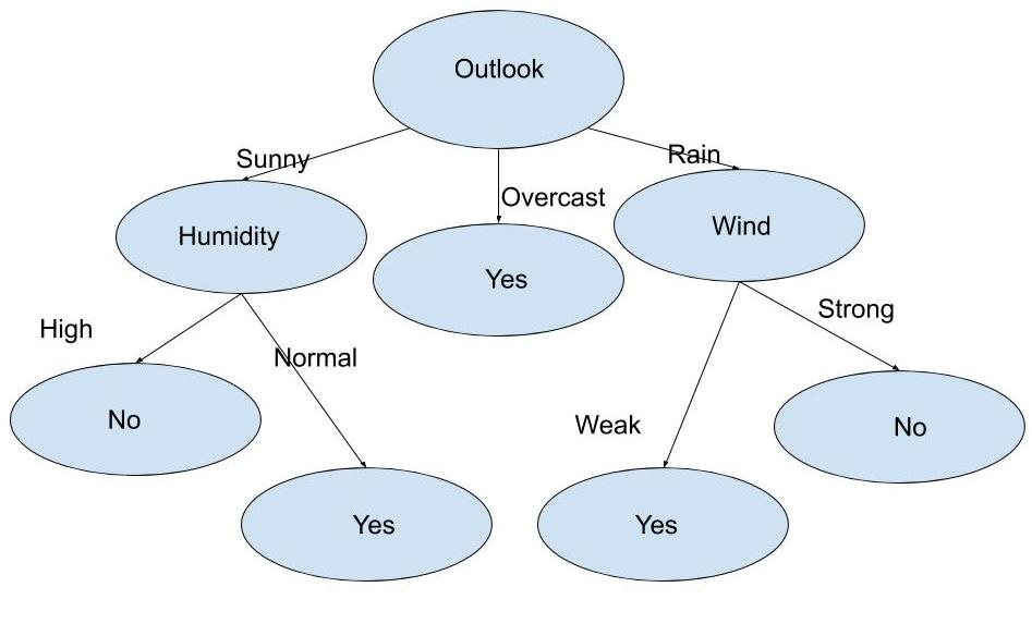
Now we will repeat the same procedure for the data with Outlook value as Sunny and for Outlook value as Rain. And do further for any remaining attribute.
At last, we will get the decision tree as
C4.5 Algorithm
This algorithm is developed by Ross Quinlan and is an extension to the ID3 Algorithm. It is suitable for solving real-world problems as it deals with both continuous and discrete attributes, missing values and pruning trees. It is quite a time-efficient.
CART Algorithm
The representation used for CART(Classification and Regression Tree) is a binary tree. Since it splits each of the input nodes into two child nodes. It generates a decision tree by employing the greedy algorithm on the training dataset to pick splits in the tree.
CHAID Algorithm
Chi-square automatic interaction detection(CHAID) builds non-binary trees for classification problems. And for regression problems it uses F-tests. It is suitable for analysing large datasets. It has gain popularity in marketing research.
MARS Algorithm
Multivariant adaptive regression splines(MARS) is a non-parametric regression technique. These are more flexible than the linear model. It is better than recursive partitioning as hinges are better for numeric data. These are similar to least-squares regression. But use when the relationship of predictor variables to the dependent variable differs over its value range.
Overfitting
We may face Overfitting while building a decision tree model. The model faces this issue when the algorithm continues to go deeper and deeper to reduce the training set error. But its results in an increased test set error. Therefore the accuracy of the model goes down. To avoid overfitting we can use two approaches:
- Pre-Pruning
- Post-Pruning
Pre-Pruning
It stops the tree construction a bit early. We should not split a node when its goodness measure is below a threshold value. But to choose an appropriate stopping point is an issue.
Post-Pruning
Firstly, it goes deeper and deeper in the tree to build a complete tree. Whenever overfitting problem arises then we do pruning as a post-pruning step. Then we use cross-validation data to check the effect of pruning. It checks whether expanding a node will make an improvement or not. If it further shows improvement, then we can continue to expand that node. But in case it shows a reduction in accuracy then we should not expand it.
Advantages of Decision Tree
- Can use for regression or classification.
- Can display it graphically.
- Highly interpretable.
- Prediction is fast.
- Features don’t need scaling.
- Ignore irrelevant features.
- Non-parametric.
- Follows the same approach as humans generally follow during decision making.
Disadvantages of Decision Tree
- Not good in performance when compared to other Supervised Machine Learning Algorithm.
- Due to overfitting we do Tuning.
- Due to the presence of highly unbalanced classes, it may not work well.
- Doesn’t work well when the dataset is very small.

Sandeep Kumar is the Founder & CEO of Aitude, a leading AI tools, research, and tutorial platform dedicated to empowering learners, researchers, and innovators. Under his leadership, Aitude has become a go-to resource for those seeking the latest in artificial intelligence, machine learning, computer vision, and development strategies.